Christian’s task
Note
This page describes the part of the implementation that was assigned to Christian. While the code implementation itself was simple, Christian contributed to many of the repositories design and strucute choices. Note for instance the advanced usage of GitHub actions for formatting, testing, building and pushing Docker images, and creating releases upon tags.
Overview
The task given was to implement a dataset that handled downloading, loading, and, preprocessing of the USPS 0 to 6 digits. The data would then be processed by a predictive framework implementing a convolutional neural network (CNN) consisting of 2 convolutional layers with a max pooling layer, using 50, \(3\times3\) filters followed by \(2\times2\) max pooling, and a rectified linear unit (ReLU) activation function. The prediction head uses a fully connected network, or multilayer perceptron (MLP) to map from the flattened feature maps to a fixed size output. To evaluate, the Recall metric was implemented.
Convolutional neural network
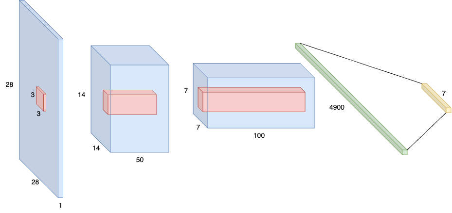
Figure 1. ChristianModel in context: The blue volumes denotes image and channel shapes, whereas red volumes denotes convolutional block filter. Each convolutional block is followed by a 2D max-pooling kernel with stride 2, and a Rectified Linear Unit (ReLU) activation function. After the second convolutional block, the data is flattened and sent through a fully connected layer which maps the flattened vector to the 7 (or num_classes) output shapes.
A standard CNN, duly named ChristianModel was implemented to process 2D image data for handwritten digit classification. Since the CNN used two convolutional layers under the hood, it was beneficial to implement a convolutional block (CNNBlock), which made the network implementation simpler. At the intersection between the convolutional and the fully connected networks—or feature extractor, and predictive network—a function find_fc_input_shape, computed the input size to the MLP using a clever trick, where a dummy image of the same size of the input is sent through the feature extractor to derive the final shape, then flattening to know what size the predictive network would need as input. This means the CNN, before initialization, is agnostic to the input size, and can in principle learn, or be used for evaluation on any 2D images, given that the initialized model has been trained on the same image shape.
Structure
ChristianModel(
  (cnn1): CNNBlock(
    (conv): Conv2d(1, 50, kernel_size=(3, 3), stride=(1, 1), padding=(1, 1))
    (maxpool): MaxPool2d(kernel_size=2, stride=2, padding=0, dilation=1, ceil_mode=False)
    (relu): ReLU()
  )
  (cnn2): CNNBlock(
    (conv): Conv2d(50, 100, kernel_size=(3, 3), stride=(1, 1), padding=(1, 1))
    (maxpool): MaxPool2d(kernel_size=2, stride=2, padding=0, dilation=1, ceil_mode=False)
    (relu): ReLU()
  )
  (fc1): Linear(in_features=4900, out_features=7, bias=True)
)
Torch summary of the network when initializing for a \(28\times28\) image with 7 output classes. Notice how the
CNNBlockonly differs by the channel mappings, and thus simplifies the implementation through abstraction. This shows the same information as in Figure 1
As per the model description, a CNN consisting of two convolutional blocks that include 2D max-pooling, and a ReLU activation function was implemented. The first convolutional block learns a mapping from a 1-channel greyscale image to 50-channel feature maps, using a \(3\times3\) convolutional kernel. The convolutional kernel uses a padding of 1, thus preserving the size of the input along the latter dimensions (height and width), but applying a 2D max pooling operation with stride 2 reduces the image size by half the original size. The second convolutional block learns a similar mapping from 50 to 100 feature maps, further halving the spatial size of the image. The feature maps are then flattened, and processed by a fully connected layer, mapping to num_classes.
United States Postal Service Dataset
Figure 2. Excerpt from USPS dataset.
The dataset implements downloading, loading, and, preprocessing of images from a subset of the United States Postal Service (USPS) dataset, corresponding to digits 0 to 6. Check the api-reference for USPSDataset0_6.
Note
While many platforms such as kaggle provide versions of the USPS dataset, they generally do not allow api-based downloading, which is required for this project. Thus, we use the official sources for downloading the training and test partitions, that come as binary, compressed, bz2-files from:
The datasets are downloaded from the official sources, processed into usable images and labels, then stored in the map-style, hierarchical HDF5 file format for ease of use. When accessing a sample, the data loader makes sure to only load a single sample at a time into memory to conserve resources, which is stated as a requirement for the assignment.
Downloading
Warning
While the requirements state that the whole dataset should not be loaded into memory at a time, for small datasets such as the USPS, a modern computer would have a easier time loading the entire dataset into memory, because of its modest image size and number of samples, totaling about 2.91 MB (train + test partitions).
Each of the partitions is accessed throughout reading the usps.h5 file, then reading a sample from either /train or /test internally in the file. The implemented USPSDataset0_6 decides which partition to load based on the argument train (boolean).
Pre-processing
Due to the collaborative nature of this project, datasets need to be capable of loading the same images but with different sizes. Thus, although the USPS dataset is constructed with \(16\times16\) image sizes in mind, other datasets such as the MNIST dataset assumes \(28\times28\) image sizes. Therefore, the dataset accepts a transform argument, which preferably should apply a sequence of Torchvision transforms, for instance using:
from torchvision import transforms
from CollaborativeCoding.dataloaders import USPSDataset0_6
transform = transforms.Compose([
    transforms.Resize((28, 28)),
    transforms.ToTensor()
])
dataset = USPSDataset0_6(
    data_path="data",
    transform=transform,
    download=True,
    train=True
)
Metric: Recall
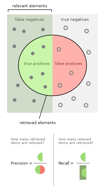
Recall, also known as sensitivity, is the subset of relevant instances retrieved, i.e., the true positives, where the predictive network made a correct prediction divided by the total number of relevant elements. In the case of multi-class prediction, that means the number of predictions the network got right, divided by the number of occurrences of the class. The keen reader will have noticed there are two possible ways of computing recall in a multi-class setting; first, the recall might be computed individually per class, then averaged over all classes, known as macro-averaging, which gives equal weight to each class; on the other hand, micro averaging aggregates the true positives and false negatives across all the classes, before calculating the metric based on the total counts, giving each instance the same weight. In this implementation of the metric, the user is able to specify which of the two types they want using the argument macro_averaging (boolean).
This project’s implementation of metrics is also the first place where Pytorch customs are broken. Where torch.nn.Module, which our metrics are inheriting from, generally advises users to rely on two interfaces. First, the class should be initialized using metric = Recall(...), then to compute the recall, one would generally expect to run recall_score = metric(y, logits), however, the group decided to store each metric, before aggregating and computing the score on an epoch-level, for more accurate computations of our metrics. While this might cause confusion for inexperienced users, we restate the age-old saying of read the docs (!).
And as such, the correct usage would instead be:
from CollaborativeCoding.metrics import Recall

metric = Recall(macro_averaging=True, num_classes=7)
...
metric(y_true, logits)

score = metric.__get_metrics__()
Where the use of a dunder method signals to the user that this should be treated as a private-class method, we provide a simpler interface through our MetricWrapper (link).
Challenges
This course focuses and requires the collaboration between multiple people, where a foundational aspect is the collaboration and interoperability of our code. This meant that a common baseline, and an agreement of the quality, and design choices of our implementation stood at the centre as a glaring challenge. However, throughout the use of inherently collaborative tools such as Git and GitHub we managed to find a common style:
When bugs are noticed, raise an issue.
The
main-branch of the GitHub repository is protected, therefore all changes must;Start out as a pull-request, preferably addressing an issue.
Pass all GitHub Actions, which meant:
Be accepted by at least one other member.
Ensure documentation using Pythons docstrings are up-to-date, following the Numpydoc style.
This structure ensured a thorough yet simple template for creating one’s implementation while adhering to the style.
Running others code
Generally, once the aforementioned requirements were set in stone and tests were implemented, other collaborators code were at such a high quality that using it was not a problem. The difficult part here is deciding on the common design choices, which we managed to do early on.
Having others run my code
As with the above conclusion, having a common ground to work from made the challenge much easier. However, upon deciding the style, there were a few disagreements to how the code should be written. But with majority voting, we were able to decide on solutions that everyone was happy with.
Tooling
While Git and GitHub were familiar to me from before, GitHub Actions, documentation using Sphinx, GitHub Packages, and the UV package manager were new to me. GitHub Actions proved to be paramount for automated testing, ensuring quality in the main branch of the project, as well as keeping code readable using formatters. Having a documentation with Sphinx, proved to be beneficial when using another persons code, and not knowing the exact internals of their implementational choices. While most collaborators started the project using miniconda, we decided to use UV as our official package manager. While I have good experience with Docker, I had not used the GitHub Container Registry (ghcr.io) before, which had the benefit of tying the container image up to the repository, and organization, instead of a single collaborator.